Shift table are required to be produced for safety measurements such as Laboratory evaluations, Electrocadiograms and Vital signs in almost all clinical studies. It displays the number of subjects with have low, normal or high test results at baseline shifted to low, normal or high results for each post baseline visit and vise verse. There’ve already been several online papers introducing how to develop shift table. However, I still strongly recommend you to read this post as it present a novel approach which is much simpler and easier for you to understand. And in this post, we will take ADLB as an example to make a demonstration.
Two types of layout for shift tables
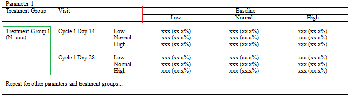
Basically, there are two kinds of layout for shift tables. In the first type, Treatment groups are placed as columns while Baseline evaluations are placed as rows.
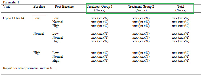
And this is the second type. You can see that the position of Treatment groups and Baseline evaluations are exchanged. Treatment groups are displayed as rows while Baseline evaluations are placed as columns.
Create sample data
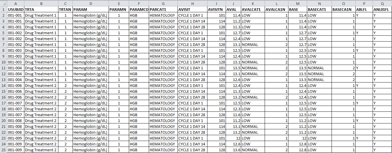
Before diving into the programming world, let’s create a sample data which can be used later for demonstration. Following shows the sample LB data stored in an excel (ADLB.xlsx) placed in D:\ drive. In our case, there are only two treatment groups.
And this block of code is for you to import above excel file into SAS dataset. Don’t forget to replace “D:\” with the full path of folder where you place the exel file – ADLB.xlsx.
Click here to hide/show code
proc import datafile=”D:\ADLB.xlsx”
out=ADLB
dbms=xlsx
replace;
sheet=”Sheet1″;
startrow=2;
getnames=Yes;
run;
Create denominator from ADSL
If you look carefully, you can see the big N in both two types of layout. This big N indicates the total number of subjects for each treatment group and can be derived from ADSL. It serves as the denominator for the percents displayed in shift table. The logic regarding how to derive big N is simple and will not be clarified in this post. Here I just want to create a dummy data which contains big N for each treatment group including total group. The data of total group is a mixture of data from all drug treatment groups and the value of TRTAN for total group will be given 3 in our case.
Click here to hide/show code
data tot;
length trta $200.;
input trta $1-6 trtan 8 tot 10-11;
cards;
Drug 1 1 8
Drug 2 2 10
Total 3 18
;
run;
Count numerator from ADLB
So far, we already have denominator, let’s go to see how to compute numerator.
First of all, we have to create total group per the layout. OUTPUT statement will be used here. It’s simple, right?
Click here to hide/show code
data adlb;
set adlb(where=(ablfl ne “Y”));
output;
trta = “Total”;
trtan = 3;
output;
run;
A lot of people would use PROC FREQ to derive the cross frequency. But I prefer PROC SQL as it is much simpler and easier. Following block of code can give you number of subjects for each unique combination of PARAM, TRTA, AVISIT, AVALCAT1 and BASECAT1. In order to manipulate data easily, numeric version those variables should be used here. For example, AVALCA1N is the numeric version of AVALCAT1.
Click here to hide/show code
proc sql;
create table mm as select paramn, param, trtan, avisitn, avisit, avalca1n, baseca1n,
count(distinct usubjid) as count from adlb
group by paramn, param, trtan, avisitn, avisit, avalca1n, baseca1n;
quit;
Due to complexity of real data, we cannot have data for all combinations required by output all the time. In order to create beautiful table and avoid us from updating code time from time, we have to create dummy data. NODUPKEY and DO loop are essential tricks here. Please note that if there are 4 groups in total, “do trtan = 1 to 3” should be replaced with “do trtan = 1 to 4”. Similarly, “do avalca1n = 1 to 3” will be replaced with “do avalca1n = 1 to 2” if there are only two values – NORMAL and ABNORMAL. In one word, you have to be careful about the digit after TO in DO statement.
Click here to hide/show code
proc sort data=mm out=dummy(keep=paramn param avisitn avisit) nodupkey; by paramn param avisitn avisit; run;
data dummy;
set dummy;
do trtan = 1 to 3;
do avalca1n = 1 to 3;
do baseca1n = 1 to 3;
count = 0;
output;
end;
end;
end;
run;
Now let’s combine dummy data and real data. Here I have to remind you that UPDATE statement can not be replaced with MERGE statement. That’s because we only want to apply update to master data which is DUMMY in our case. If the value of COUNT in MM is different from that in DUMMY, the value of COUNT in DUMMY will be overwritten by that from MM. Otherwise, value of COUNT in DUMMY will be left as 0.
Click here to hide/show code
proc sort data = mm; by paramn param trtan avisitn avisit avalca1n baseca1n; run;
proc sort data = dummy; by paramn param trtan avisitn avisit avalca1n baseca1n; run;
data mm;
update dummy mm;
by paramn param trtan avisitn avisit avalca1n baseca1n;
run;
By far, we have got all numerators including 0. Below block of code can help you merge numerator and denominator together and then compute percents. SUBPAD function is applied here for alignment of decimal points.
Click here to hide/show code
proc sql undo_policy=none;
create table mm as select a.*, b.tot, b.trta from
mm as a left join tot as b
on a.trtan = b.trtan;
quit;
data mm;
length pct $200.;
set mm;
pct = right(subpad(strip(put(count,best.)),1,2))||” (“||right(subpad(strip(put((count/tot)*100,8.1)),1,5))||”%)”;
run;
Tranpose data per layout
With all required percents available, we can move forward to transfrom data so that data can be displayed as required by our layout.
First layout
Let’s go back and take a look at the first layout. In the first layout, Baseline evaluations should be displayed as rows. Therefore, BASECA1N related variable will be placed in ID statement in PROC TRANSPOSE procedure. TREATMENT group variable as well as AVALCAT1 will be placed in BY statement.
Click here to hide/show code
data mm;
length col1-col3 $200.;
set mm;
id = baseca1n + 3;
col1 = strip(trta);
col2 = strip(propcase(avisit));
if avalca1n = 1 then col3 = “Low”;
else if avalca1n = 2 then col3 = “Normal”;
else if avalca1n = 3 then col3 = “High”;
run;
proc sort data = mm; by paramn param trtan col1 avisitn col2 avalca1n col3 id; run;
proc transpose data = mm out=final(drop=_name_) prefix=col;
by paramn param trtan col1 avisitn col2 avalca1n col3;
id id;
var pct;
quit;
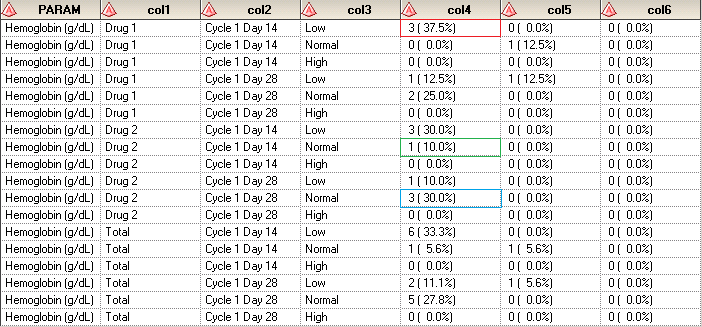
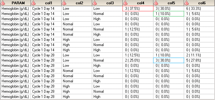
Here is the result output. There are 3 subjects having LOW test evaluation at Baseline shifted to LOW at Cycle 1 Day 14 visit. The total number of subjects from Drug 1 treatment is 8 and 3/8 is 37.5%. Only 1 subject in Drug 2 treatment get LOW test evaluation at Baseline and then shift to NORMAL at Cycle 1 Day 14 visit.
Second layout
In the second layout, TREATMENT group should be displayed as rows. Therefore, TREATMENT related variable will be placed in ID statement in PROC TRANSPOSE procedure. BASECAT1 (BASECA1N) variable as well as AVALCAT1 (AVALCA1N) will be placed in BY statement.
Click here to hide/show code
data mm;
length col1-col3 $200.;
set mm;
id = trtan + 3;
col1 = strip(propcase(avisit));
if baseca1n = 1 then col2 = “Low”;
else if baseca1n = 2 then col2 = “Normal”;
else if baseca1n = 3 then col2 = “High”;
if avalca1n = 1 then col3 = “Low”;
else if avalca1n = 2 then col3 = “Normal”;
else if avalca1n = 3 then col3 = “High”;
run;
proc sort data = mm; by paramn param avisitn col1 baseca1n col2 avalca1n col3 id; run;
proc transpose data = mm out=final(drop=_name_) prefix=col;
by paramn param avisitn col1 baseca1n col2 avalca1n col3;
id id;
var pct;
quit;
Here is the result output for second layout. If you compare it against that for the first layout, you would find that numbers are matched. For example, the numbers in red square are the same. They are all equal to “3 (30.0%)”.
Like the post? Welcome to share or you can subscribe to get latest post. How to subscribe? Go to the top-right corner of this web page to submit your name and email address.