Previously, we have introduced how to apply two sample test using SAS. What if we need to compare means between k (k >= 2) samples? Perhaps you will suggest that multiple two-sample t-test can be used. However, this will increase the type I error rate (please refer to the end of this post for details). This post will present you one way ANOVA and how to apply ANOVA using PROC AVOVA and PROC GLM.
Assumptions of One Way ANOVA
- Normality – Samples should be normally of approximately normally distributed.
- Independence – Samples must be independent from each other.
- Homogeneity of variance – Variances of the samples should be equal.
One Way ANOVA Hypotheses
One way Analysis of Variance (ANOVA) can be used to determine whether there are any statistically significant differences between the means of three or more independent groups. It test the null hypothesis:
![]()
µ is group mean for different groups while k is equal to total number of groups. The alternative hypothesis is that at least two group means are statistically significant different from each other.
Calculations of One Way ANOVA
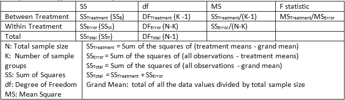
In essence, the ratio of Variance between treatment and Variance within treatment should be calculated. By comparing this ratio to a handbook value, we can determine the statistical significance. Variance between treatment is just Mean Square between treatment while variance within treatment is Mean Square within treatment. Each Mean Square is just the Sum of Squares divided by its degree of freedom. And F ratio is in essense the ratio of Mean Squares. Follow figure shows you how to compute three types of Sum of Squares.
Decision Rule
If the computed F statistics is greater than the F critical value within k-1 numerator and N-K denominator degrees of freedom, we can reject the null hypothesis. In other words, we can consider that at least two group means are statistically signicant from each other if p-value is less than 0.05. So far, the ANOVA only tells you all group means are not statistically significant equal. It does not tell you where the difference lies. For further multiple comparison, we still need Scheffe’s or Tukey test.
SAS procedures that can be applied for One Way ANOVA
Both ANOVA procedure and GLM procedure can be applied to perform analysis of variance. PROC ANOVA is preferred when the data is balanced (refer to the end of this post for details) as it is faster and uses less storage than PROC GLM. Besides balanced data, PROC ANOVA can also be used for these situations: one way analysis of variance, Latin square designs, certain partially balanced incomplete block design, completely nested desings, and designs with cell frequencies that are proportional to each other and also proportional to he background population. When the data is unbalanced, PROC GLM should be applied. In this case, PROC ANOVA is forbidden to be applied.
Example using PROC ANOVA for balanced Data
First of all, let’s use below code to create a dummy data which will be used later for demonstration. After submiting below code to SAS, you will get a dataset named ADXL which contains three variables: TRTA, TRTAN and AVAL.
Click here to hide/show code
data adxl;
input trta $ aval @@;
if trta = “Placebo” then trtan = 1;
else if trta = “Drug50” then trtan = 2;
else trtan = 3;
datalines;
Placebo 19.4 Placebo 32.6 Placebo 27.0 Placebo 32.1 Placebo 33.0
Placebo 17.7 Placebo 24.8 Placebo 27.9 Placebo 25.2 Placebo 24.3
Drug50 17.0 Drug50 19.4 Drug50 9.1 Drug50 11.9 Drug50 15.8
Drug50 20.7 Drug50 21.0 Drug50 20.5 Drug50 18.8 Drug50 18.6
Drug100 14.3 Drug100 14.4 Drug100 11.8 Drug100 11.6 Drug100 14.2
Drug100 17.3 Drug100 19.4 Drug100 19.1 Drug100 16.9 Drug100 20.8
;
run;
Here is the code for overall ANOVA analysis and multiple comparison using Turkey’s test. CLDIFF option can enable SAS to present results of TUKEY option as confidence intervals for all pairwise differences between means.
Click here to hide/show code
proc sort data=adxl; by trtan trta; run;
ods trace on;
ods output OverallANOVA = OverallANOVA CLDiffs = CLDiffs;
proc anova data=adxl;
class trtan;
model aval = trtan;
means trtan / tukey cldiff;
run;
ods output close;
ods trace off;
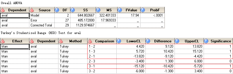
After submitting above code to SAS, you can get two datasets named OverallANOVA and CLDiffs. They are all displayed in below figure. You can see that ProbF is less than 0.0001 which suggests that we should reject the null hypothesis and consider that at least two group means are significantly different from each. The bottom panel shows the results of multiple comparion using Turkey’s test. Means from Drug50 and Drug100 are not significantly different. And means from any treatment group – no matter if it is Drug50 or Drug100 – and Placebo are significantly different.
Example using PROC GLM
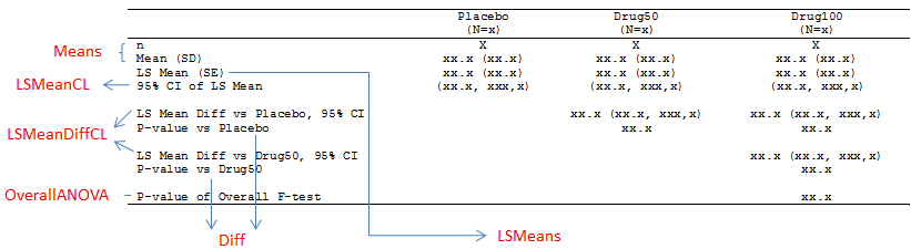
In real world, data in clinical industry is not balanced and we have to apply PROC GLM. Here we still use above dummy data because PROC GLM can be applied to both types of data: balanced and unbalanced. Suppose that we’d like to create a table like below, we need to get number of observations, arithmetic mean, LS mean, differences of LS mean and corresponding SD, SE, 95% CI and p-value.

Here is the initial code that most of us would apply. There is nothing wrong except LSMENAS statement. It requests all pairwise differences.
Click here to hide/show code
proc sort data = adxl; by trtan; run;
ods trace on;
ods output Means = Means OverallANOVA = OverallANOVA
LSMeans = LSMeans
LSMeanDiffCL = LSMeanDiffCL LSMeanCL = LSMeanCL;
proc glm data=adxl;
class trtan;
model aval = trtan;
means trtan;
lsmeans trtan/pdiff cl stderr;
run;
ods output close;
ods trace off;
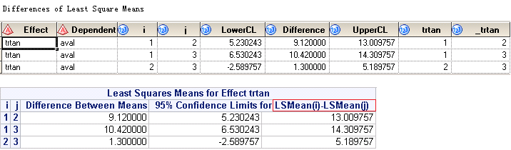
If you submit above code, you will get something like below. The upper panel is from output dataset named LSMeanDiffCL while the lower panel is from listing window. You can see that, the differences is not what we want as we’d like to have LSMean from Drug50 minus LSMean from Placebo. If you look at the figure closely, it gives you LSMean from Placebo minus LSMean from Drug50.
To fix this problem, we can apply below code. But there are repetitions in your output datasets LSMeans and LSMeanCL. And you have to apply PROC NODUPKEY when transforming and dealing with your data. Here the first LSMEANS statement specifies the ‘1’ level of TRTAN is the control and the second LSMEANS statement specifies the ‘2’ level of TRTAN is the control.
Click here to hide/show code
proc sort data = adxl; by trtan; run;
ods trace on;
ods output Means = Means OverallANOVA = OverallANOVA
LSMeans = LSMeans
LSMeanDiffCL = LSMeanDiffCL LSMeanCL = LSMeanCL Diff = Diff;
proc glm data=adxl;
class trtan;
model aval = trtan;
means trtan;
lsmeans trtan/tdiff pdiff=control(“1”) cl stderr;
lsmeans trtan/tdiff pdiff=control(“2”) cl stderr;
run;
ods output close;
ods trace off;
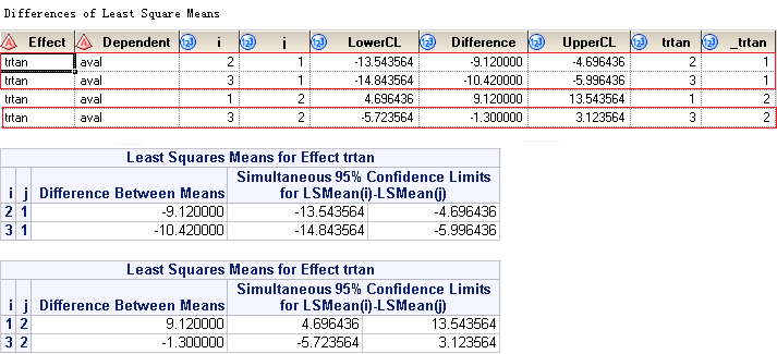
Below figures shows the output dataset named LSMeanDiffCL and corresponding results printed to your listing window. Rows surrounded in red box are what we exactly need per our table shell.
Finally, here is the figure shows you from which output datasets you can find the required info for our table.


nice practicesing examples.