In our last post, we only showed you how to use LSMEAN statement to compute LSMEAN and differences of LSMEAN. Today in this post, we will introduce the other two statements: CONTRAST and ESTIMATE. This two statements can also help you reach the goal. Before knowing how to use those two statements, we have to learn the statistical assumption of PROC GLM and how the coefficient matrix will be constructed.
Statistical Assumption for using PROC GLM
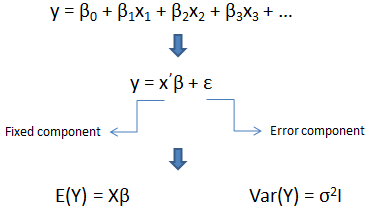
The “GLM” stands for General Linear Model. The basic statistical assumption underlying the least squares approach to general linear modeling is that the observed values of each dependent variable can be written as the sum of two parts: a fixed component and a random noise or error component. In our following figure, y is dependent variable while x1, x2, x3 … are independent variables. Y is vector of dependent variable values while X is the matrix of independent coeffcients, I is the identity matrix and σ2 is the common variance for the errors. Here I need your attention that fixed component is a linear function of the independent coefficients. These independent coefficients X are costructructed from the model effects.
Specification of Effects and Types of Model
Each term in a model is called an effect which is a variable or combination of variables. Effects are specified with a special notation using variable names and operators. The variables in the model can be categorized into two types: classification variables and continous variables. As for the operators, there are two primary kinds: crossing, nesting. The bar operator which can be used to shorten the specification will not be introduced here. In the analysis-of-variance model, classfication model should be declared in the CLASS statement. Continous variables can be used as response variables and covariates. Suppose that A, B, C are CLASS variables while y1, y2, x and z are continous variables. Here shows you how to specify effects for different types of model.
| Specification | Type of Model |
| Model y = x; | Simple regression |
| Model y = x z; | Multiple regression |
| Model y = x x*x; | Polynomial regression |
| Model y1 y2 = x z; | Multivariate regression |
| Model y = a; | One-way ANOVA |
| Model y = a b c; | Main-effects ANOVA |
| Model y = a b a*b; | Factorial ANOVA with interaction |
| Model y = a b(a) c(b a); | Nested ANOVA |
| Model y1 y2 = a b; | Mutivariate analysis of variance (MANOVA) |
| Model y = a x; | Analysis of covariance |
| Model y = a x(a); | Separate-slopes regression |
| Model y = a x x*a; | Homogeneity-of-slopes regression |
Parameterization of PROC GLM Models
As I have told you in the first section of this post that PROC GLM constructs a linear model according to the specification in the MODEL statement. Each effect in the MODEL statement generates one or more columns in a design matrix X. Here we only presents you four commonly used effects, Other effects such as Nested effects, Continuous-Nesting-Class Effects, Continuous-by-class Effects, General Effects will not be described here.
Intercept
All models include a column of 1s by default to estimate an intercept parameter µ. NOINT option can be used to suppress the intercept.
Regression Effects
Values of regresion Effects (covariates) will be copied into the design matrix directly.
Main Effects
If a classfication variable has m levels, PROC GLM generates m columns in the design matrix for it main effect. Each column represents one of the levels of the classification variable. The default order of the columns is the sort order of the values of their levels. And this order can be controlled with the ORDER = option in the PROC GLM statement.
Suppose that there are two main effects A and B. A has two levels while B has three levels. The left part of below table shows different kinds of combination of levels of effect A and effect B. The right part of table shows how the matrix is constructed for each combination. A good understanding of this can enable you to use CONTRAST and ESTIMATE statements correctly.
| Data | Design Matrix | |||||||
| A | B | |||||||
| A | B | µ | A1 | A2 | B1 | B2 | B3 | |
| 1 | 1 | 1 | 1 | 0 | 1 | 0 | 0 | |
| 1 | 2 | 1 | 1 | 0 | 0 | 1 | 0 | |
| 1 | 3 | 1 | 1 | 0 | 0 | 0 | 1 | |
| 2 | 1 | 1 | 0 | 1 | 1 | 0 | 0 | |
| 2 | 2 | 1 | 0 | 1 | 0 | 1 | 0 | |
| 2 | 3 | 1 | 0 | 1 | 0 | 0 | 1 | |
Crossed Effects
For crossed effects, order of the terms is determined by order of the variables in the CLASS statement. For example, B*A becomes A*B if A precedes B in the CLASS statement.
| Data | Design Matrix | |||||||||||||
| A | B | A*B | ||||||||||||
| A | B | µ | A1 | A2 | B1 | B2 | B3 | A1B1 | A1B2 | A1B3 | A2B1 | A2B2 | A2B3 | |
| 1 | 1 | 1 | 1 | 0 | 1 | 0 | 0 | 1 | 0 | 0 | 0 | 0 | 0 | |
| 1 | 2 | 1 | 1 | 0 | 0 | 1 | 0 | 0 | 1 | 0 | 0 | 0 | 0 | |
| 1 | 3 | 1 | 1 | 0 | 0 | 0 | 1 | 0 | 0 | 1 | 0 | 0 | 0 | |
| 2 | 1 | 1 | 0 | 1 | 1 | 0 | 0 | 0 | 0 | 0 | 1 | 0 | 0 | |
| 2 | 2 | 1 | 0 | 1 | 0 | 1 | 0 | 0 | 0 | 0 | 0 | 1 | 0 | |
| 2 | 3 | 1 | 0 | 1 | 0 | 0 | 1 | 0 | 0 | 0 | 0 | 0 | 1 | |
CONTRAST statement and ESTIMATE statement
CONTRAST statement enables you to perform custom hypothesis tests by specifying an L vector or matrix for testing the univariate hypothesis Lβ = 0 or the multivariate hypothesis LBM = 0. Here is the syntax for CONTRAST statement.
| CONTRAST ‘label’ effect values <… effect values>/<options> | |
| label | Identifies the estimate on the output. Label is required for every contrast specified and labels must be enclosed in quotes. |
| effect | Identifies an effect that appears in the MODEL statement or the INTERCEPT effect. |
| Values | Are constants that are the elements of the L vector associated with the preceding effect. |
| E option | Displays the entire L vector. This option is useful in confirming the ordering of parameters for specifying L. |
ESTIMATE statement enables you to estimate linear function of the parameters by multiplying the vector L by the parameter estimate vector b, resulting Lb. Here is the syntax for ESTIMATE statement.
| ESTIMATE ‘label’ effect values <… effect values>/<options> | |
| label | Identifies the estimate on the output. Label is required for every contrast specified and labels must be enclosed in quotes. |
| effect | Identifies an effect that appears in the MODEL statement or the INTERCEPT effect. |
| Values | Are constants that are the elements of the L vector associated with the preceding effect. |
| E option | Displays the entire L vector. This option is useful in confirming the ordering of parameters for specifying L. |
Demontration using real case
Here we still use dummy data from our last post. It will get you a dataset named ADXL which contains three variables: TRTA, TRTAN and AVAL.
Click here to hide/show code
data adxl;
input trta $ aval @@;
if trta = “Placebo” then trtan = 1;
else if trta = “Drug50” then trtan = 2;
else trtan = 3;
datalines;
Placebo 19.4 Placebo 32.6 Placebo 27.0 Placebo 32.1 Placebo 33.0
Placebo 17.7 Placebo 24.8 Placebo 27.9 Placebo 25.2 Placebo 24.3
Drug50 17.0 Drug50 19.4 Drug50 9.1 Drug50 11.9 Drug50 15.8
Drug50 20.7 Drug50 21.0 Drug50 20.5 Drug50 18.8 Drug50 18.6
Drug100 14.3 Drug100 14.4 Drug100 11.8 Drug100 11.6 Drug100 14.2
Drug100 17.3 Drug100 19.4 Drug100 19.1 Drug100 16.9 Drug100 20.8
;
run;
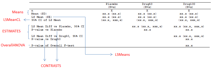
And we also copy our target table shell here to refresh your mind.

Here will still use PROC GLM to compute the required statistics. Now let’go back to our Parameterization section and see how the matrix will be designed given that there is only on classfication effect. Since there are three levels and there will be three columns.
| Data | Design Matrix | |||
| TRTAN | TRTAN1 | TRTAN2 | TRTAN3 | |
| 1 | 1 | 0 | 0 | |
| 2 | 0 | 1 | 0 | |
| 3 | 0 | 0 | 1 | |
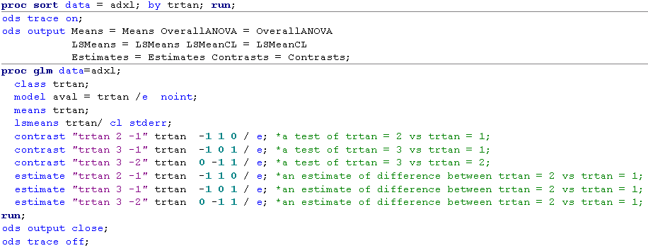
Below figure shows you how to specify CONTRAST and ESTIMATE statement to test or estimate the difference of between two levels. Let’s take trtan = 2 vs trtan = 1 as an example, the first level and the second level will be the first column and second column in the design matrix. Therefore, effect values like -1 1 0 should be used in both CONTRAST and ESTIMATE statement.
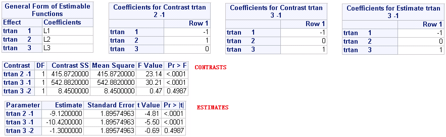
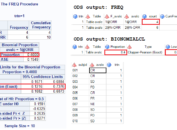
After submitting above code, you will get below results. The results are in consistent with that we have have got using LSMEAN statement. Here I have to remind you that CONTRAST statement can be omitted if ESTIMATE statement is used here as the p-value can also be provided by ESTIMATE statement.
At last, here still shows you from which output datasets to retrieve the require information. Please note that %95 CI for LS Mean Diff is not available from above code. We have to use PROC MIXED or apply LSMEANS statement in PROC GLM.
LSMEAN vs ESTIMATE Statment
| LSMEAN | ESTIMATE |
| When estimate a given effect, all levels of this effect will be given | Can estimate a given level of a given effect |
| Estimate differences of lsmean through diff option | Estimate differences of LSMEAN through specifications |


good,
how to calculate population bioequivalence in sas and excel
Will try to do that later in future.